It’s the time to say good bye to Vlookup and start using Index & Match.
One of the staff has asked me to fetch a last transaction value and the corresponding field for a given parameter. The first answer for the solution is a Vlookup, however it has a variety of limitations
1. Your data range is limited to a table. That means the data you are looking up has to be in a standard tabular form. You cannot use VLOOKUP to find a lookup value in a different table, sheet, or offset row. This limits the ways you can display your data, as anything you want to lookup must be available in a standard table format in your spreadsheet.
2. VLOOKUP always searches the leftmost column of the specified table to find the lookup value. Again, this limits your choices in presenting data as lookup values always have to be to the left of the return values. This sometimes means you must have multiple copies of tables in order, think far ahead when creating tables that might be used in lookup, or reorder columns after the fact simply to use VLOOKUP.
3. You can only specify the return value column by index number. This means there is no way to include a static reference to the return value column. If someone adds a column between the lookup value column and return value column, it will break your VLOOKUP and you have to manually increase the column index number in the formulas. This is a maintenance nightmare.
4. VLOOKUP provides a very limited approximate match feature. The only aproximate match option finds the nearest “less than” value. Unless you want that type of behavior, you’re out of luck and can’t use it.
5. By default, VLOOKUP uses approximate match. If this is how you want it to function, then great… However, in many cases you want an exact value returned. It gives no indication it is picking a closest match result. If you do not want this behavior (which is most of the time, I have found…), you remember to explicitly set the Range_lookup argument in the formula to FALSE. Range_lookup is optional, and not a very descrive name of this feature, so it is often overlooked. This quirk is exasperated by the second danger…
6. VLOOKUP can provide false results if the table is not sorted in ascending order! This is an issue when you use the approximate match feature, which is TRUE by default. Basically, VLOOKUP starts at the top of the table and goes down row by row until to gets to a valie less than or equal to the lookup value. If your table is not sorted in ascending order, this can give false results, as the formula stops processing rows immediately after finding a “match.”
The answer to these problems and limitations is the INDEX-MATCH lookup method. This methods uses two functions together to provide a more safe and flexible lookup feature. Here’s how each function works, independently:
- INDEX returns the value at the intersection of a row and column in a given range.
- Formula: =INDEX(Array, Row_num, Column_num)
- Array - The range of cells
- Row_num - The row to return data from
- Column_num – The column to return the data from [optional]
-
- MATCH returns a position of an item in an array that matches a value.
- Formula: =MATCH(Lookup_value, Lookup_array, Match_type)
- Lookup_value – The value you want to find in the lookup value array
- Lookup_array – The range containing lookup values
- Match_type – Exact (0), Nearest Less Than (-1), or Nearest Greater Than (1) [optional]
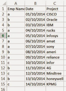
Here is the problem statement,
Data Set

Required

Lets also understand CSE Formula
Last date 
Last project 
Any clarification reach me back venu@vnv.ca


